Making a chart on the fly

I posted a map on social media recently that drew wholly from online resources; I’m trying to do this for all my charts and maps this quarter. There are practical reasons, having to do with not keeping large data files lying around; there are also principled reasons, having to do with reproducible research and adherence to community standards.

I learned to do this mainly by taking Kieran Healy’s invaluable Data Wrangling and Data Visualization course, online.

I am, I hope, as sensitive as anyone to historians’ need to consult archival and arcane resources and I love the library as much as anyone. But if a reasonably authoritative chart or map for teaching can be made from community resources, it probably should be.

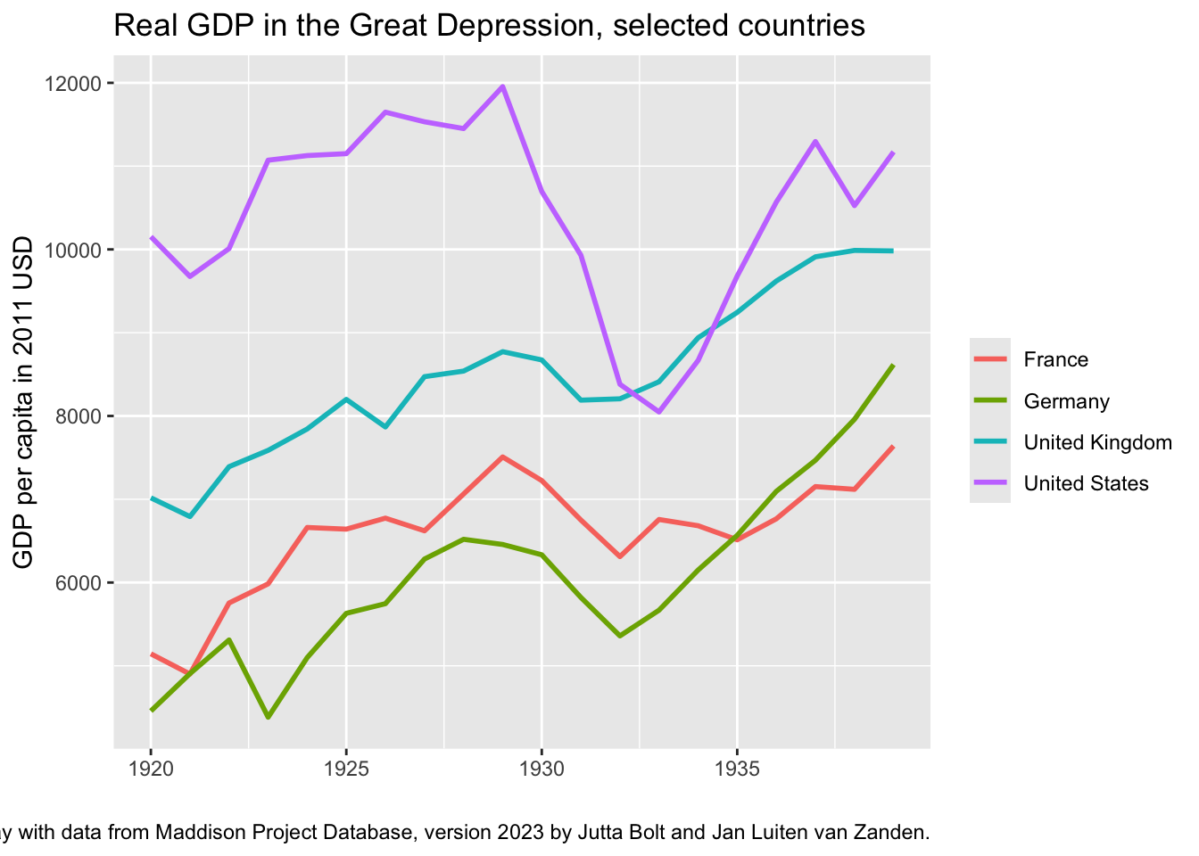
So here’s an example; I often like to show something like the comparative impact of the Great Depression. You could go to the library and look in International Historical Statistics and type information by hand into a spreadsheet—and I wouldn’t want to stop you. But you could also reach out and grab information from, let’s say, the Maddison Project at the University of Groningen.¹

## make a list of packages we will use
packages <- c("tidyverse", "haven")
## install the packages not already installed
install.packages(setdiff(packages, rownames(installed.packages())))
## make the code available for this exercise
lapply(packages, "library", character.only=TRUE)
## Read data from the University of Groningen Maddison Project
read_dta(file = "https://dataverse.nl/api/access/datafile/421303") |>
  filter(year > 1919 & year < 1940) |> ## limit data to interwar years
  filter(country == "Germany" | ## select some industrial countries
           country == "France" |
           country == "United Kingdom" |
           country == "United States") -> data ## store data
## now let's plot the data
data |>
  ggplot() +
  geom_line(aes(x = year, 
                y = gdppc, 
                group = country, 
                color = country),
            linewidth = 1) +
  labs (
    x = "", y = "GDP per capita in 2011 USD",
    color = "", 
    caption = "Chart made using R and ggplot by Eric Rauchway with data from Maddison Project Database, version 2023 by Jutta Bolt and Jan Luiten van Zanden.",
    title = "Real GDP in the Great Depression, selected countries"
  ) -> p ## store this graph in an object called "p"---we'll want it again in a second
## now, display the object called "p"
p 

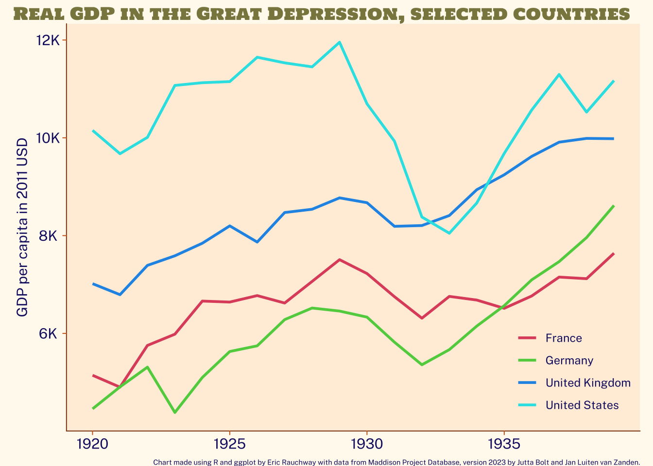
Everything else is aesthetics.

## some code packages for prettification
more_packages <- c("showtext", "ggtext", "scales", "grafify")
## install these packages not already installed
install.packages(setdiff(more_packages, rownames(installed.packages())))
## make this code available for this exercise
lapply(more_packages, "library", character.only=TRUE)
## get some fonts from google
font_add_google(name = "Public Sans", family = "Public Sans")
font_add_google(name = "Holtwood One SC", family = "Holtwood One SC")
showtext_auto()
## make some choices for how we want the graph to look
theme_set(
  theme_void() +
    theme(
      text = element_text(family = "Public Sans", 
                          color = "midnightblue"),
      plot.title = element_markdown(family = "Holtwood One SC", 
                                    color = "khaki4"),
      plot.title.position = "plot",
      plot.caption = element_markdown(size = rel(0.5)),
      plot.background = element_rect(fill = "floralwhite",
                                     color = "floralwhite"),
      plot.margin = margin(l=10,r=10),
      axis.text = element_text(margin = margin(2,2,2,4)),
      axis.title.y = element_text(angle = 90, margin =
                                    margin(2,2,4,2)),
      axis.line = element_line(color = "chocolate4"),
      axis.ticks = element_line(color = "chocolate3"),
      axis.ticks.length = unit(1, "mm"),
      legend.position = "inside",
      legend.justification.inside = c(0.98, 0.05),
      panel.background = element_rect(fill = "antiquewhite1",
                                      color = "NA")
    )
)

## now, make the plot again, but with these aesthetic choices, calling up the object "p" where we stored the plot before
p +
  scale_color_grafify(palette = "r4") + ## a color-blind-friendly palette
  scale_y_continuous(labels = label_number(scale_cut = cut_short_scale()))

So the key here is, none of this data or even, in this example, the fonts live on my computer, or the server; it’s all pulled from the web. Which means you could copy the code and run it on your computer, in some environment supporting R, and it should work the same.

Footnotes

1. See Jutta Bolt and Jan Luiten van Zanden, “Maddison-Style Estimates of the Evolution of the World Economy: A 2023 Update,” Journal of Economic Surveys, 2024, 1--41. I had the good fortune to sit next to Maddison at dinner once. He was a very pleasant conversationalist. This ranks up there, for data nerdery, with the times I’ve had dinner with a PI of American National Election Studies and with a co-director of Correlates of War.